
A Deep Dive into Skewed Joins, GroupBy Bottlenecks, and Smart Strategies to Keep Your Spark Jobs Flying
How to Diagnose, Prevent, and Fix Performance Bottlenecks from Skewed Data in Your Spark Workloads

Data skew in Apache Spark refers to an uneven distribution of data across partitions, often manifesting during shuffle-intensive operations like joins or group-by aggregations. In a skewed scenario, one or a few partitions end up holding far more records for a particular key than others, leading to hotspots and straggler tasks. This imbalance causes performance bottlenecks (tasks processing heavy partitions take much longer) and inefficient resource usage (some executors sit idle). In extreme cases, heavily skewed partitions can even exhaust executor memory and cause job failures. Below, we delve into why skew occurs in joins and aggregations, and provide comprehensive strategies—ranging from Spark configuration tweaks to code-level patterns and architectural designs—to alleviate data skew.
Why Data Skew Occurs in Joins and Aggregations
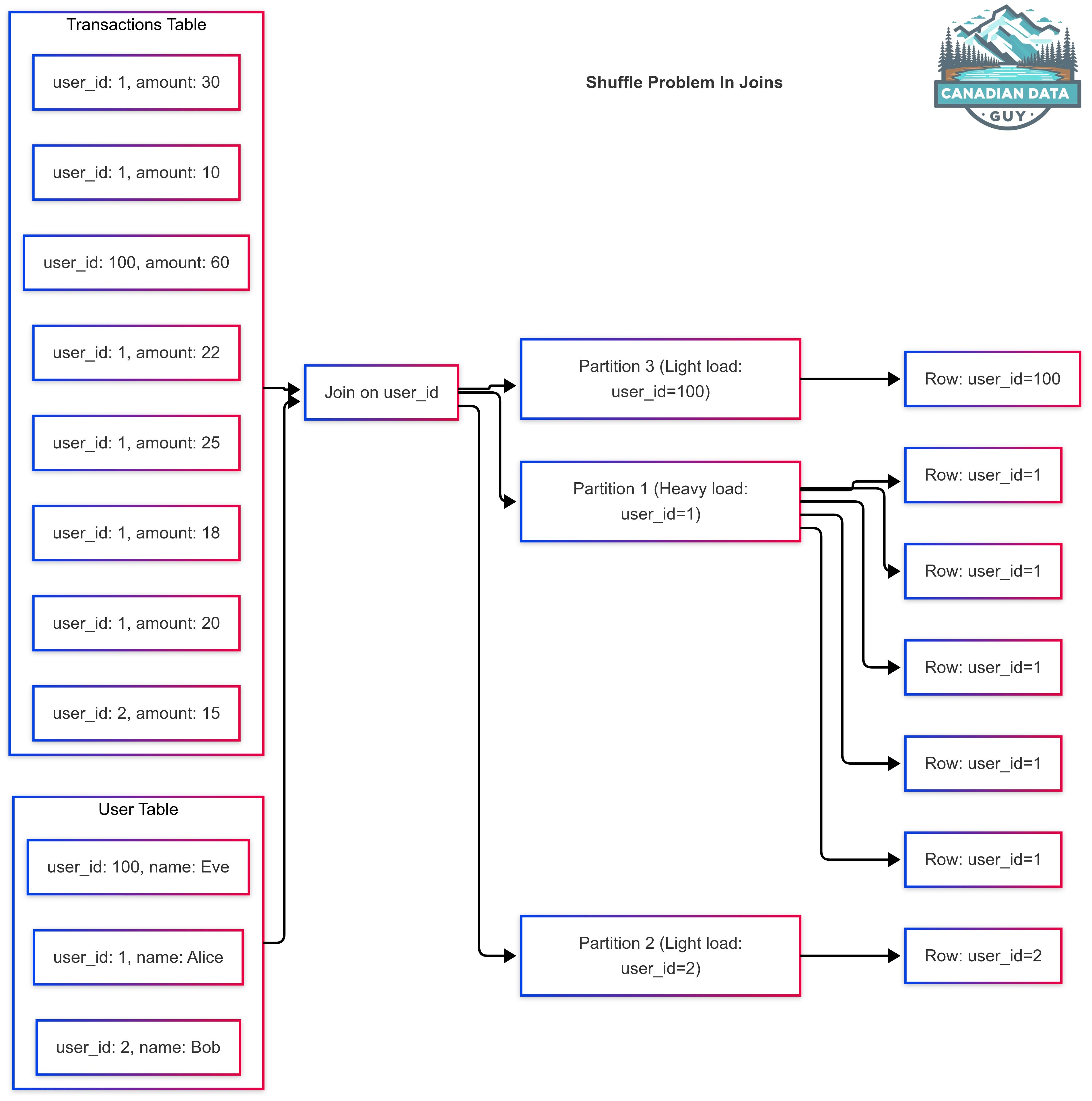
Join Operations: In Spark (excluding broadcast joins), joining two datasets on a key requires redistributing data so that records with the same key end up on the same partition (for a shuffle hash join or sort-merge join). If the key distribution is highly uneven (e.g. one key value appears in 90% of the records), the partition handling that key will be massive compared to others, causing skew. All records for that popular key funnel into one task, creating a severe load imbalance. For example, consider joining a large transactions table with a user table on user_id when a few “power users” have the vast majority of transactions. The join partition corresponding to those user_ids will handle hundreds of thousands of records, while other partitions process only a few – resulting in stragglers and possibly out-of-memory errors.
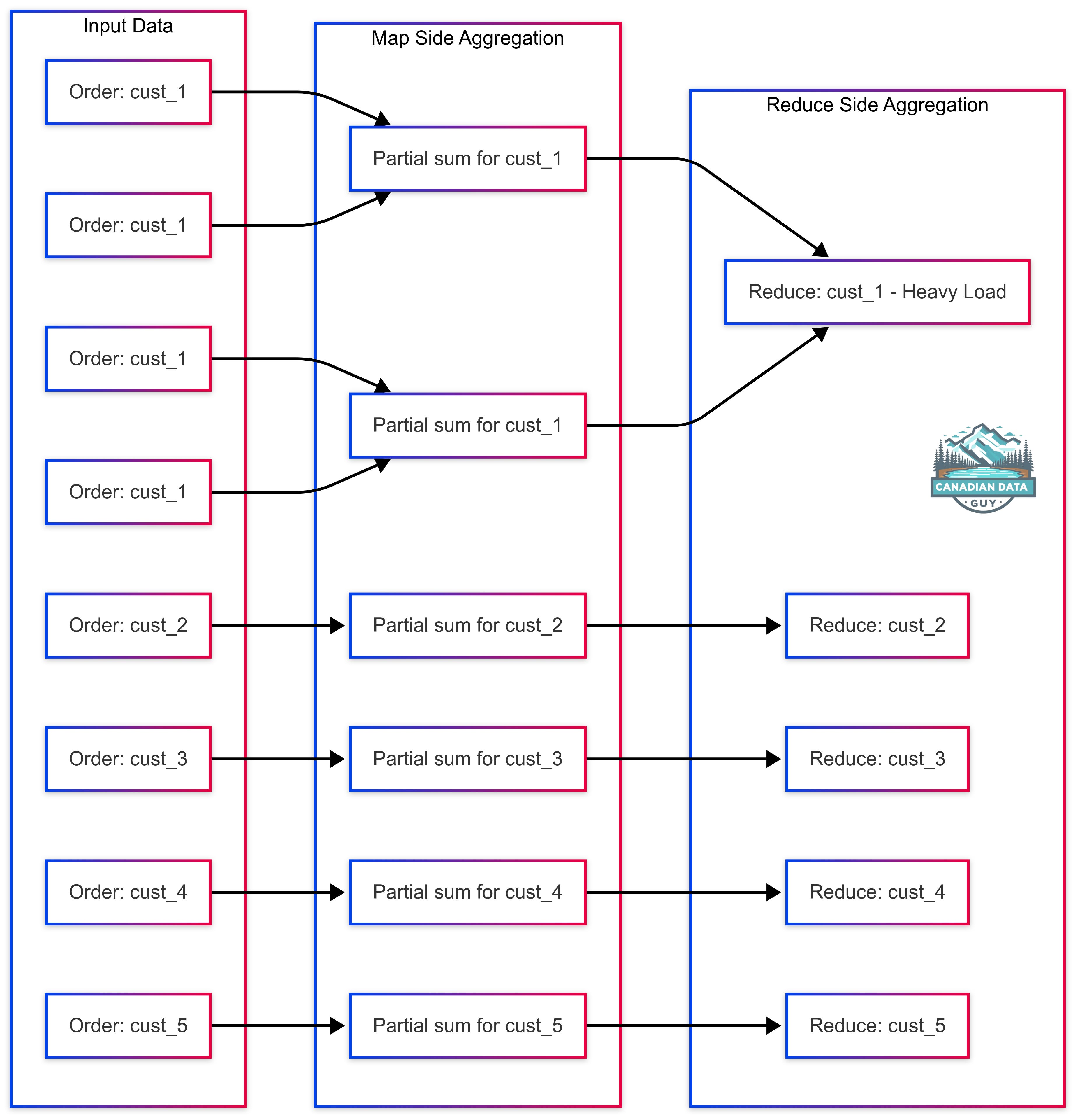
GroupBy and Aggregations: Similarly, grouping or aggregating by a key brings all data for each key onto one executor. If some keys occur far more frequently than others, those keys’ partitions become disproportionately large. For instance, a groupBy("customer_id") on an orders dataset where a handful of customers account for most orders will produce skew: the reducer for those popular customers must aggregate an extremely large list, while others handle trivial amountsl. Even though Spark performs map-side partial aggregation, a single reduce task will still have to combine all intermediate results for a heavy key, leading to one very slow task.
Understanding these root causes guides us to solutions. Next, we address join skew and groupBy/aggregation skew separately, discussing targeted techniques for each.
How do we know if we have a Skew Problem?
To identify if there is a skew problem in Spark, several indicators and methods can be employed:
Task Duration Discrepancy:
If all tasks in a shuffle stage finish except for a few that hang for a long time, this may indicate data skew.
Spark UI Analysis:
Check the tasks summary metrics in the Spark UI. A significant difference between the minimum and maximum shuffle read sizes can suggest skewness.
Data Spills:
If, despite tuning the number of shuffle partitions, there are numerous data spills, this might point to data skew.
Row Count Disparity:
Counting rows grouped by join or aggregation columns can reveal skew. A significant difference in row counts for different groups indicates potential skew issues.
Compression Ratios:
Highly compressed tables can affect the estimation of shuffle partitions, leading to spills. Monitoring this can help identify such cases.
Mitigating Skew in Join Operations
When joining two datasets on a key, Spark must shuffle records so that identical keys end up on the same partition. If one key is heavily overrepresented, its partition can become a bottleneck. Below are strategies ordered from most to least recommended
1. Adaptive Query Execution (AQE) – Automatic Skew Handling
Spark 3.0+ introduced Adaptive Query Execution (AQE), which can dynamically detect and correct skewed partitions during runtime. When AQE is enabled, Spark measures the size of each shuffle partition after the initial shuffle. If it finds any partition that is both exceptionally large in absolute terms and multiple times larger than the median partition size, it automatically splits that partition into smaller sub-tasks and replicates the corresponding rows from the other side of the join so each sub-task can run independently.
How It Works
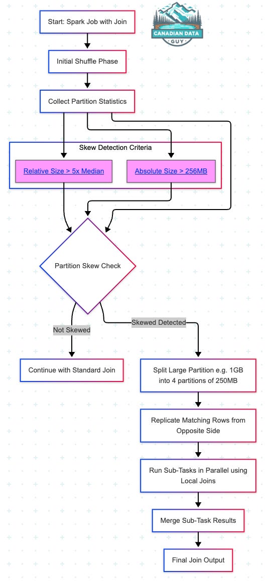
Collect Partition Statistics:
After the shuffle phase, Spark records the size (bytes) of every partition on both sides of the join.
Identify Skewed Partitions:
A partition is marked as “skewed” only if it meets both criteria:Absolute‐Size Threshold:
spark.sql.adaptive.skewJoin.skewedPartitionThresholdInBytesDefault:256MBRelative‐Size Factor:
spark.sql.adaptive.skewJoin.skewedPartitionFactor(Default:
5.0)
If the median shuffle‐partition size is 50 MB, a factor of 5.0 means any partition > 250 MB qualifies—provided it also exceeds the 256 MB absolute threshold.
Split & Replicate:
Suppose partition #17 is 1 GB and the coalesced‐partition target is 250 MB. Spark divides that 1 GB into four ~250 MB sub-partitions.
For a join, each of those sub-partitions must still see all matching rows from the opposite dataset. Spark duplicates those matching rows N times (once per sub-partition) so each sub-task can run a local join.
Run Subtasks in Parallel & Merge Results:
Instead of a single, massive task pulling 1 GB, Spark launches N tasks (e.g., four tasks pulling ~250 MB each plus replicated rows).
When those sub-tasks finish, Spark concatenates their outputs to produce the final joined result.
Because this splitting and replication occur after the initial shuffle—when Spark has accurate sizes—no query rewriting or manual “hints” are required.
Configuration
# Enable AQE (on by default in Spark 3.2+)
spark.sql.adaptive.enabled=true

# Enable skew-join correction
spark.sql.adaptive.skewJoin.enabled=true

# Absolute-size threshold for skewed partitions
spark.sql.adaptive.skewJoin.skewedPartitionThresholdInBytes=256MB

# Relative-size factor: if a partition is > factor × median size, it's skewed
spark.sql.adaptive.skewJoin.skewedPartitionFactor=5.0

# (Spark 3.3+) Force AQE to apply skew-join splitting even if it adds shuffle overhead
spark.sql.adaptive.forceOptimizeSkewedJoin=true
Pros & Cons
Pros:
Zero code changes: No query rewrites, no manual hints.
Runtime intelligence: Works on any sort-merge or shuffle-hash join where skew is severe.
Eliminates straggler tasks without requiring you to identify skewed keys in advance.
Cons:
Applies only to shuffle joins (sort-merge and shuffle-hash). Broadcast joins never shuffle, so they aren’t “skewed.”
Splitting and replicating can introduce extra shuffle I/O; mild skew might not trigger or be worth splitting.
You may need to tune thresholds (
skewedPartitionThresholdInBytesandskewedPartitionFactor) to avoid splitting on nearly-skewed partitions.
Keep This Post Discoverable: Your Engagement Counts!
Your engagement with this blog post is crucial! Without claps, comments, or shares, this valuable content might become lost in the vast sea of online information. Search engines like Google rely on user engagement to determine the relevance and importance of web pages. If you found this information helpful, please take a moment to clap, comment, or share. Your action not only helps others discover this content but also ensures that you’ll be able to find it again in the future when you need it. Don’t let this resource disappear from search results — show your support and help keep quality content accessible!
2. Broadcast Hash Join (Small–Large Optimization)
If one side of a join is small enough to fit in memory on every executor, a broadcast hash join eliminates virtually all skew risk. By broadcasting the smaller dataset to every executor, Spark can join on the large side without shuffling it by key. Even a “hot” key on the large side is processed in parallel across many tasks, because each task already has the complete, in-memory copy of the smaller table.
How It Works
Spark Optimizer Picks It Automatically (if small side ≤ 10 MB by default):
Controlled by:
spark.sql.autoBroadcastJoinThreshold(Default:10MB)Raise this value to allow larger small tables but not more than 1 GB practically
Explicitly Force Broadcast in DataFrame Code:
from pyspark.sql.functions import broadcast

result = largeDF.join(broadcast(smallDF), "joinKey")
Spark SQL Hint:
SELECT /*+ BROADCAST(s) */ *
FROM large l
JOIN small s
  ON l.joinKey = s.joinKey;
Since the large dataset is not shuffled by key, no single reducer processes all rows for a heavy key. Instead, each task hashes the broadcasted small side in-memory, and streams its assigned partitions of the large side through that hash.
Pros & Cons
Pros:
No shuffle on large side—completely eliminates skew related to the small side.
Simple to implement via
broadcast()hints or by tuningspark.sql.autoBroadcastJoinThreshold.Dramatic speedups when one side is truly small and the other side has a hot key.
Cons:
The “small” table must fit comfortably in each executor’s memory. If it’s too large (hundreds of MB), broadcasting can create memory pressure or OOM.
Not applicable when both sides are large.
Total cluster memory usage for the small table = (# executors) × (size of small table).
3. Handling Skewed Keys Separately (Divide & Conquer)
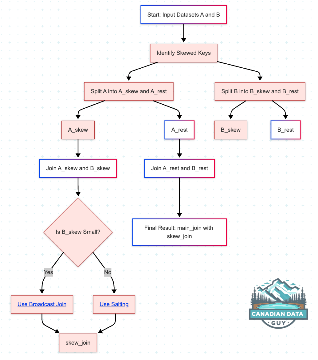
If you know exactly which key(s) are skewed, you can split your data into two subsets—the skewed-key subset and the “rest”—process them separately, then recombine
How It Works
Split Each Dataset into “Skewed” vs. “Rest”:
skewed_keys = ["USA"]

# Dataset A (large or small, doesn’t matter)
A_skew   = A.filter(F.col("country") == "USA")
A_rest   = A.filter(F.col("country") != "USA")

# Dataset B
B_skew   = B.filter(F.col("country") == "USA")
B_rest   = B.filter(F.col("country") != "USA")
Join the “Rest” Subsets Normally:
main_join = A_rest.join(B_rest, "country")Since “USA” is removed, these partitions will be balanced—assuming no other keys are extremely skewed.
Join the “Skewed” Subsets Separately with an Optimized Strategy:
If
B_skewis small enough, broadcast it:
skew_join = A_skew.join(broadcast(B_skew), "country")Otherwise, you could salt only the “USA” key (as shown above) or use any other technique.
Union the Two Results:
final_result = main_join.unionByName(skew_join)Pros & Cons
Pros:
Simplicity: Process the skewed key in isolation; non-skewed data is untouched.
You choose exactly how to handle the problematic key (e.g., broadcast, salt, or extra resources).
No need to change logic for the majority of keys.
Cons:
Requires an extra read/scan (filter) on each dataset—though filter is usually cheap.
Increases job complexity: two join operations instead of one.
If more than one key is skewed, you must repeat this process for each key or group of keys—still subject to skew within that sub‐subset.
Must identify skewed key(s) beforehand.
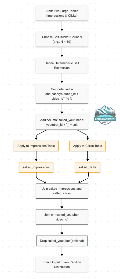
4. Salting Every Key (Uniform Distribution Across N Buckets)
In real-world joins—especially at scale—any single key with extremely high cardinality (for example, a superstar YouTuber like “mr_beast”) can overwhelm one partition, leading to severe performance bottlenecks. While you might compensate by detecting and salting just that one “hot” key, a more robust approach is to uniformly salt every youtuber_id, ensuring that even unexpected popularity spikes are handled gracefully. By applying a deterministic salt to all keys, each youtuber_id is augmented with a bucket index, distributing its rows across up to N partitions. Matching rows from both tables still join correctly because the salt is derived deterministically from the join key (and potentially another column like video_id).
How It Works
Choose a Salt Count (N)
Decide how many buckets to split every
youtuber_idinto (for example,N = 10).Aim for each salted partition to be on the order of 100–300 MB (or your target). Use the Spark UI’s “Shuffle Read Size by Task” to gauge ideal bucket size.
Compute a Deterministic Salt for Each Row
For each row, compute:
salt = abs(hash(concat(youtuber_id, video_id))) % N
salted_youtuber = CONCAT(youtuber_id, "_", salt)
This ensures:
All rows belonging to the same (youtuber_id, video_id) produce the same
(salted_youtuber, video_id)pair in both tables.Every youtuber_id is split across up to N buckets—popular keys will spread widely, less-popular keys may cluster in fewer buckets if they have fewer distinct
video_idvalues.
3. Salt Both Tables in PySpark
import pyspark.sql.functions as F

N = 10

def saltAllExpr(yid_col, vid_col):
    """
    Deterministic salt for every (youtuber_id, video_id):
    salted_youtuber = youtuber_id + "_" + (abs(hash(youtuber_id || video_id)) % N)
    """
    return F.concat(
        yid_col,
        F.lit("_"),
        (F.abs(F.hash(F.concat(yid_col, vid_col))) % N).cast("string")
    )

# Salt the IMPRESSIONS table
salted_impressions = impressions.withColumn(
    "salted_youtuber",
    saltAllExpr(F.col("youtuber_id"), F.col("video_id"))
)

# Salt the CLICKS table
salted_clicks = clicks.withColumn(
    "salted_youtuber",
    saltAllExpr(F.col("youtuber_id"), F.col("video_id"))
)
Every
(youtuber_id, video_id)pair gets a consistent bucket index in[0..9].For
"mr_beast"withvideo_id = "abc123",salted_youtuber = "mr_beast_4"(for example).A different video
"xyz789"might map to"mr_beast_7".A less-popular youtuber with only one or two videos may occupy only 1–2 buckets—but that’s fine.
Perform the Salted Join
joined = salted_impressions.alias("imp").join(
    salted_clicks.alias("clk"),
    on=[ "salted_youtuber", "video_id" ],
    how="inner"
)
Before salting: All
"mr_beast"rows (across anyvideo_id) would land in a single partition.After salting: Each distinct
(youtuber_id, video_id)combination goes to a bucketyoutuber_id_<0..9>, so"mr_beast"content spreads across up to 10 partitions—one per bucket index.This eliminates a single “hot” partition for
"mr_beast".
Spark SQL Equivalent
WITH salted_impressions AS (
  SELECT
    *,
    CONCAT(
      youtuber_id,
      '_',
      CAST(ABS(hash(CONCAT(youtuber_id, video_id))) % 10 AS STRING)
    ) AS salted_youtuber
  FROM impressions
),
salted_clicks AS (
  SELECT
    *,
    CONCAT(
      youtuber_id,
      '_',
      CAST(ABS(hash(CONCAT(youtuber_id, video_id))) % 10 AS STRING)
    ) AS salted_youtuber
  FROM clicks
)
SELECT
  imp.*,
  clk.viewer_id,
  clk.timestamp AS click_timestamp
FROM salted_impressions imp
JOIN salted_clicks clk
  ON imp.salted_youtuber = clk.salted_youtuber
 AND imp.video_id       = clk.video_id;
Each
(youtuber_id, video_id)deterministically maps to one of 10 buckets.Even if
"mr_beast"has 100 videos, those 100 distinct(youtuber_id, video_id)pairs spread across up to 10 buckets.
Pros & Cons
Pros:
Uniform Distribution for All Keys
Any youtuber with many videos—like"mr_beast"—will spread its rows across N buckets.No Conditional Logic on “Hot” Keys
You don’t need to first identify which youtuber is skewed; every key is salted uniformly.Deterministic
Matching(youtuber_id, video_id)always end up in the same bucket on both sides, so joins remain correct.Works for Any Join
Applies whether one or both tables are large—no reliance on broadcast.
Cons:
Extra Shuffle Volume
Every row in both tables carries an extra salted key, and all rows must shuffle by(salted_youtuber, video_id).If a youtuber is lightly used, its rows may end up in only one or two buckets—but they still shuffle.
If data was quite balanced originally, salting “everything” may introduce more shuffle than strictly necessary.
Choosing the Right N Is Crucial
If N is too small, heavily skewed keys (like
"mr_beast") still concentrate too much data in one bucket.If N is too large, you create many small partitions, which increases scheduler overhead.
Need to Drop
salted_youtuberAfter the Join
If you only care about the original key (youtuber_id), dropsalted_youtuberonce the join is done.
When to Use “Salt Everything”
Use this approach when:
You don’t know in advance which keys will be skewed (e.g., an Uber driver of the week suddenly goes viral, or any youtuber’s popularity spikes).
Data volume is large and dynamic, and you want a one‐size‐fits‐all solution rather than conditionally checking for hot keys.
You want consistent distribution for all
(youtuber_id, video_id)pairs without maintaining a list of skewed keys.
Additional Considerations (Ideally; try to avoid getting into these)
Tuning Shuffle Partitions
Adjust: spark.sql.shuffle.partitions to a value higher than the default (200), ideally a few times your cluster’s total cores, so that partitions remain small. Too many partitions cause scheduler overhead; too few cause each partition to be large.
Speculative Execution: Enabling speculation (spark.speculation=true) can alleviate the impact of skew by attempting to re-run straggling tasks on another executor. This doesn’t fix the skew itself, but if a task is slow (perhaps due to skew or maybe a slow node), Spark will launch a duplicate task elsewhere. Whichever finishes first wins. In a skew scenario, a speculated task is still doing the same heavy work, so it won’t magically complete faster unless the original executor was anomalously slow. However, speculation can sometimes help if, say, one executor was busy with garbage collection while another could do the work faster – it provides a safety net for stragglers. It’s generally good to enable in large clusters, but note it causes extra resource usage for those duplicate tasks.
Monitoring with the Spark UI
In the Stages tab, expand a SQL stage and click Physical Plan.
Under Shuffle Read Size by Task, look for a single bar that towers over the others—that’s your skewed partition.
Use those insights to decide between AQE or manual salting.
Filtering Out Problematic Rows
If certain values (e.g.,
NULLor outliers) cause extreme skew but are not essential, you can drop them before the join, Only do this if you can accept losing those rows from the result.
cleanedDF = originalDF.filter(F.col("country").isNotNull())Use Skew Hints (Spark 3.4+)
You can annotate specific keys as skewed in a Spark SQL query so that Spark generates a plan that avoids shuffling them into a single reducer
Memory and Shuffle Tuning: While not fixing skew, you might need to adjust memory configs to handle it. For instance, if one partition is huge, increasing executor memory or shuffle buffer sizes (spark.shuffle.spill.numElementsForceSpillThreshold, spark.shuffle.file.buffer, etc.) won’t solve the skew but might prevent OOM crashes by allowing Spark to spill gracefully. Similarly, ensure spark.memory.fraction or spark.sql.autoBroadcastJoinThreshold are set such that the heavy data can be handled (e.g., give more memory to shuffle if needed). These are more about coping with skew than removing it.
Adaptive Query Execution (AQE): As discussed, ensure spark.sql.adaptive.enabled=true (should be default on modern Spark) and spark.sql.adaptive.skewJoin.enabled=true. You can adjust spark.sql.adaptive.skewJoin.skewedPartitionFactor (default 5) and ...skewedPartitionThresholdInBytes (default 256MB) to tune how aggressively Spark flags partitions as skewed Lowering these values makes Spark split smaller skews, but setting them too low might cause unnecessary splitting. In Spark 3.3+, if you really want to force skew join handling, spark.sql.adaptive.forceOptimizeSkewedJoin=true will apply the optimization even if it might add extra shuffle overhead.
Tackling Skew in Spark Aggregations: From Simple Sums to Semi-Additive Metrics
Aggregation operations like groupBy().agg() in Spark can become major performance bottlenecks when data is skewed. A small number of high-cardinality keys can result in uneven workload distribution, where one reducer is overloaded while others remain idle. While Spark's map-side partial aggregation helps, it alone can’t prevent reducers from becoming overwhelmed when skewed keys funnel massive data into single tasks.
In this deep dive, we’ll explore practical patterns to mitigate skew during aggregations, especially focusing on semi-additive metrics like averages, distinct counts, and ratios—metrics that can't always be merged as trivially as sums or counts.
1. Two-Stage Aggregation with Salting
The most effective method for aggregation skew is a two-stage salted aggregation. In the first stage, you add a salt (random or deterministic) to the key, distributing rows across more groups. In the second stage, you aggregate these partials back to the original key.
How It Works:
Add a new column (e.g.,
salt = rand() % N) to the grouping keyGroup by
(key, salt)and compute partial aggregatesRe-group by
keyto merge the partials
PySpark Example:
from pyspark.sql.functions import col, rand, floor, sum as _sum, count as _count

N = 10
salted_df = df.withColumn("salt", floor(rand() * N))

# First stage: partial aggregation
partial = salted_df.groupBy("key", "salt").agg(
    _sum("value").alias("partial_sum"),
    _count("value").alias("partial_count")
)

# Second stage: final aggregation
final = partial.groupBy("key").agg(
    _sum("partial_sum").alias("total_sum"),
    _sum("partial_count").alias("total_count")
)
This works well for semi-additive metrics like average:
final.withColumn("avg", col("total_sum") / col("total_count"))Pros:
Greatly reduces skew on hot keys
Flexible: works for sums, counts, averages, etc.
Cons:
Not directly applicable to non-associative metrics (like median, percentile)
Requires an extra stage of aggregation and data shuffle
You must choose N carefully
2. Favor Combiner-Friendly DataFrame Operations
In the DataFrame API, Spark automatically performs map-side combine for aggregation functions like sum, count, and avg. This significantly reduces data shuffled across the network.
Best Practices:
Avoid collecting all values per key using
collect_listorcollect_setunless neededPrefer built-in aggregation functions that support partial aggregation
Example:
df.groupBy("user_id").agg(
    _sum("impressions").alias("total_impressions"),
    _count("clicks").alias("click_count")
)
This automatically benefits from map-side combine.
3. Hierarchical or Incremental Aggregation
Instead of grouping by the final key directly, first group on a compound key (e.g., key + day), then roll up to the main key. This acts like salting but uses a meaningful secondary attribute.
Example: Group by (customer_id, date), then group again by customer_id.
Pros:
Uses natural structure in data
More interpretable than random salt
Cons:
Only works if meaningful secondary keys exist
Adds complexity to query logic
4. Isolate Skewed Keys
When just a few keys are skewed (e.g., "mr_beast" on YouTube), isolate them:
Filter the skewed keys
Aggregate them separately
Aggregate the rest normally
Union results
Pros:
Simple logic for non-skewed keys
You can fine-tune treatment of skewed keys
Cons:
Manual, doesn’t scale to many skewed keys
Separate logic paths = more complexity
Special Note: Semi-Additive Metrics
For metrics like averages, ratios, or distinct counts, special care is needed:
Average: Use partial sums and counts, then divide
Ratios: Keep numerator/denominator separate, aggregate both, then divide
Count Distinct: Use
approx_count_distinct()for scalable approximations
Some metrics cannot be split and recombined (e.g., exact percentiles). In those cases, use isolation or rethink the need for exact aggregation.
Final Thoughts for Aggregates
Aggregation skew is an invisible killer in Spark jobs. The best strategy is proactive design: salt heavy keys, use partial aggregation, and always choose APIs that favor combiners. With these patterns, even semi-additive or tricky metrics can be made scalable at massive volumes.
If you're dealing with skew, don't just throw resources at it. Design for it.
Summary of Recommendations for Joins
Recommended first Adaptive Query Execution (AQE): Zero code changes, runtime splitting for any sort-merge or shuffle-hash join.
Broadcast Hash Join
When one side is small (≤ 10 MB by default to 1GB). Hint in DataFrame or SQL.
Avoids all skew because no shuffle on the small side.
Salting the Key
When neither side is small, but you know exactly which key(s) dominate.
Manual, but guaranteed to split a hot key across N partitions.
Handle Skewed Keys Separately
When you can isolate a small number of skewed keys.
Split data into “skewed” vs. “rest”; optimize skewed subset, then union.
By applying these strategies in order—starting with AQE’s automatic handling, then broadcasting small tables, and, if necessary, resorting to manual salting or custom partitioning—you can eliminate or dramatically reduce skew-related stragglers in your Spark join operations. Choose the approach that best fits your cluster’s Spark version, data volume, and the complexity you’re willing to maintain.
Architectural Patterns and Data Design to Reduce Skew
Beyond individual Spark jobs, you can sometimes address skew at the data architecture level to prevent issues before they happen:
Skew-Aware Data Partitioning: As discussed, designing how data is partitioned or bucketed in storage can reduce skew. For example, if you frequently group or join by a key that’s skewed, consider storing the data partitioned by that key and a secondary split. A real-world practice: if one category of data is 90% of the dataset, you might partition that category’s data further by another field. Essentially, acknowledge the skewed key in your data model and subdivide it. This could mean separate tables or partitions for heavy categories. When you process the data, you then handle those partitions in parallel. The benefit is you're not repeatedly shuffling the entire dataset to discover the same skew; you’ve pre-divided it.
Pre-Aggregation / Summaries: If your use-case allows, maintain rolling aggregates for skewed keys. For instance, if one user has a million events per day and you always compute their daily total, consider updating a running total for that user in a database or a separate file, rather than recomputing from scratch in each Spark job. By reducing the raw data volume for that key through prior aggregation, you avoid the huge shuffle for that key at query time. This is applicable in pipelines where data is appended incrementally (common in streaming or daily ETL). You trade off storage (keeping summary data) for performance.
Alternate Algorithms: In some cases, you might choose a different approach entirely. For example, for a skewed distinct count, using an approximate algorithm (like HyperLogLog) per partition can avoid bringing all data together. Or using Bloom filters to reduce data before join (filter out records that won’t match). These are specific to certain problems but can mitigate skew by cutting down the data processed.
Scaling Up Hot Data Separately: This is more of an infrastructure pattern – if one key’s data is massive, you could route that to a specialized system. For instance, maybe that one key corresponds to a particular customer – you could give them their own dedicated processing or database, and exclude those records from the general Spark workflow. It’s an extreme solution, but sometimes separating concerns (multi-tenancy isolation) helps if one tenant’s data skews the whole system.
Monitoring and Iteration: A softer “pattern” is to continuously monitor your Spark job metrics (especially in Spark UI or via logs) to catch skew issues and then adjust. Over time, you may adapt your data ingestion or job logic to handle new skewed keys as data grows. For example, if a new user becomes a power user, you might add them to the “skewed key list” for salting. In practice, skew patterns can change, so an architecture that can adjust (or a code path that can automatically detect top N heavy keys and treat them differently) can be very useful.
In essence, architectural approaches are all about not putting all eggs in one basket – distribute data smartly from the ground up, and treat the outliers with special care. This reduces the burden on any single Spark job to handle an immense skew on the fly.
Thank you for such a detailed explanation on solution options for handling data skew.
However, I have a question, probably a quick one...
Given that now we also have Liquid Clustering feature available in Databricks, should Liquid Clustering be considered as the first and the foremost recommended solution, even over the AQE please?
In other words, as a recommended approach, shouldn't Liquid Clustering be considered first, followed by AQE, then BroadcastHashJoin, then Salting.
Please correct me if I'm wrong in my understanding.
Great stuff, thanks for sharing!